Tutorial
Step 1: Setup
# Install PyPEEC
#   - With a Python environment
#   - With a Conda environment

# Check the PyPEEC version
pypeec --version

# Extract the PyPEEC examples
pypeec examples examples

# Extract the PyPEEC documentation
pypeec documentation documentation
Step 2: Introduction
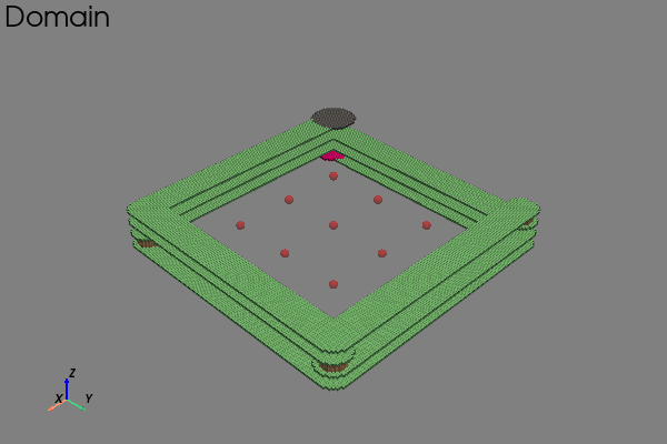
This tutorial demonstrates how PyPEEC can be used to simulate a four-layer PCB coil.
The coil has two terminals and the simulation is done in the frequency domain.
All the commands are executed inside the virtual environment from the examples folder.

Geometry of the considered four-layer PCB coil.
Step 3: Mesher
# Run the mesher from the command line
#   - geometry.yaml - contains the geometry description (input)
#   - voxel.json.gz - contains the meshed voxel structure (output)

pypeec mesher \
    --geometry tutorial/geometry.yaml \
    --voxel tutorial/voxel.json.gz
# Run the mesher from the Python interpreter
#   - geometry.yaml - contains the geometry description (input)
#   - voxel.json.gz - contains the meshed voxel structure (output)

import pypeec

file_geometry = "tutorial/geometry.yaml"
file_voxel = "tutorial/voxel.json.gz"

pypeec.run_mesher_file(
    file_geometry=file_geometry,
    file_voxel=file_voxel,
)
00:00:00.00 : pypeec   : info     : load the input data : start
00:00:00.08 : pypeec   : info     : load the input data : done
00:00:00.08 : pypeec   : info     : load the mesher
00:00:06.90 : pypeec   : info     : run the mesher
00:00:06.90 : pypeec   : info     : check the input data
00:00:06.91 : pypeec   : info     : mesher_shape : enter : 00:00:00.00
00:00:06.91 : pypeec   : debug    :     prepare the shapes
00:00:06.91 : pypeec   : debug    :         parse the layers
00:00:06.92 : pypeec   : debug    :         create the shapes
00:00:06.96 : pypeec   : debug    :         get the voxel size
00:00:06.96 : pypeec   : debug    :         merge the shapes
00:00:07.06 : pypeec   : debug    :     voxelize the shapes
00:00:07.35 : pypeec   : debug    :         domain = trace / size = 19728
00:00:07.35 : pypeec   : debug    :         domain = via / size = 1195
00:00:07.35 : pypeec   : debug    :         domain = src / size = 361
00:00:07.35 : pypeec   : debug    :         domain = sink / size = 361
00:00:07.35 : pypeec   : info     : mesher_shape : exit : 00:00:00.44
00:00:07.35 : pypeec   : info     : voxel_point : enter : 00:00:00.00
00:00:07.35 : pypeec   : debug    :     check_cloud = True
00:00:07.35 : pypeec   : debug    :     filter_cloud = True
00:00:07.35 : pypeec   : debug    :     original number = 25
00:00:07.42 : pypeec   : debug    :     final number = 25
00:00:07.42 : pypeec   : info     : voxel_point : exit : 00:00:00.07
00:00:07.42 : pypeec   : info     : voxel_resampling : enter : 00:00:00.00
00:00:07.42 : pypeec   : debug    :     use_reduce = False
00:00:07.42 : pypeec   : debug    :     use_resample = False
00:00:07.42 : pypeec   : debug    :     original number = 331056
00:00:07.42 : pypeec   : debug    :     final number = 331056
00:00:07.42 : pypeec   : info     : voxel_resampling : exit : 00:00:00.00
00:00:07.42 : pypeec   : info     : voxel_conflict : enter : 00:00:00.00
00:00:07.43 : pypeec   : info     : voxel_conflict : exit : 00:00:00.00
00:00:07.43 : pypeec   : info     : voxel_integrity : enter : 00:00:00.00
00:00:08.24 : pypeec   : info     : voxel_integrity : exit : 00:00:00.81
00:00:08.24 : pypeec   : info     : voxel_summary : enter : 00:00:00.00
00:00:08.24 : pypeec   : debug    :     voxel size
00:00:08.24 : pypeec   : debug    :         n = (132, 132, 19)
00:00:08.24 : pypeec   : debug    :         d = (3.50e-05, 3.50e-05, 3.50e-05)
00:00:08.24 : pypeec   : debug    :         s = (4.63e-03, 4.63e-03, 6.65e-04)
00:00:08.24 : pypeec   : debug    :         c = (1.94e-03, 1.94e-03, 0.00e+00)
00:00:08.24 : pypeec   : debug    :         A = (2.14e-05, 3.08e-06, 3.08e-06)
00:00:08.24 : pypeec   : debug    :     voxel summary
00:00:08.24 : pypeec   : debug    :         V_total = 1.42e-08
00:00:08.24 : pypeec   : debug    :         V_used = 9.12e-10
00:00:08.24 : pypeec   : debug    :         n_total = 331056
00:00:08.24 : pypeec   : debug    :         n_used = 21215
00:00:08.24 : pypeec   : debug    :         ratio = 6.41e-02
00:00:08.24 : pypeec   : debug    :         n_domain = 4
00:00:08.24 : pypeec   : debug    :         n_component = 1
00:00:08.24 : pypeec   : debug    :         n_cloud = 25
00:00:08.24 : pypeec   : debug    :     voxel domain
00:00:08.24 : pypeec   : debug    :         trace = 19298
00:00:08.24 : pypeec   : debug    :         via = 1195
00:00:08.24 : pypeec   : debug    :         src = 361
00:00:08.24 : pypeec   : debug    :         sink = 361
00:00:08.24 : pypeec   : info     : voxel_summary : exit : 00:00:00.00
00:00:08.24 : pypeec   : info     : successful mesher termination
00:00:08.24 : pypeec   : info     : save the results : start
00:00:08.67 : pypeec   : info     : save the results : done
Step 4: Viewer
# Run the viewer from the command line
#   - voxel.json.gz - contains the meshed voxel structure (input)
#   - viewer.yaml - contains the plot configuration (input)
#   - tag_plot - list of plots to be shown (defined in viewer.yaml)
#   - plot_mode - method used for rendering the plots

pypeec viewer \
    --voxel tutorial/voxel.json.gz \
    --viewer config/viewer.yaml \
    --tag_plot domain voxelization adjacent \
    --plot_mode qt
# Run the viewer from the Python interpreter
#   - voxel.json.gz - contains the meshed voxel structure (input)
#   - viewer.yaml - contains the plot configuration (input)
#   - tag_plot - list of plots to be shown (defined in viewer.yaml)
#   - plot_mode - method used for rendering the plots

import pypeec

file_voxel = "tutorial/voxel.json.gz"
file_viewer = "config/viewer.yaml"

pypeec.run_viewer_file(
    file_voxel=file_voxel,
    file_viewer=file_viewer,
    tag_plot=["domain", "voxelization", "adjacent"],
    plot_mode="qt",
)
Plot showing the different domains composing the voxel structure.
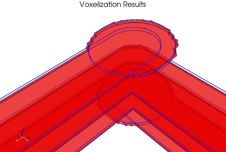
Plot comparing the voxelized and original geometries.
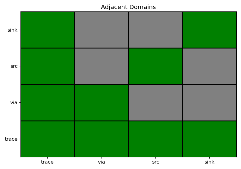
Plot showing which domains are adjacent to each others.
Step 5: Solver
# Run the solver from the command line
#   - voxel.json.gz - contains the meshed voxel structure (input)
#   - problem.yaml - contains the magnetic problem description (input)
#   - tolerance.yaml - contains the solver numerical tolerances (input)
#   - solution.json.gz - contains the problem solution (output)

pypeec solver \
    --voxel tutorial/voxel.json.gz \
    --problem tutorial/problem.yaml \
    --tolerance config/tolerance.yaml \
    --solution tutorial/solution.json.gz
# Run the solver from the Python interpreter
#   - voxel.json.gz - contains the meshed voxel structure (input)
#   - problem.yaml - contains the magnetic problem description (input)
#   - tolerance.yaml - contains the solver numerical tolerances (input)
#   - solution.json.gz - contains the problem solution (output)

import pypeec

file_voxel = "tutorial/voxel.json.gz"
file_solution = "tutorial/solution.json.gz"
file_problem = "tutorial/problem.yaml"
file_tolerance = "config/tolerance.yaml"

pypeec.run_solver_file(
    file_voxel=file_voxel,
    file_problem=file_problem,
    file_tolerance=file_tolerance,
    file_solution=file_solution,
)
00:00:00.00 : pypeec   : info     : load the input data : start
00:00:00.10 : pypeec   : info     : load the input data : done
00:00:00.10 : pypeec   : info     : load the solver
00:00:01.07 : pypeec   : info     : run the solver
00:00:01.07 : pypeec   : info     : check the input data
00:00:01.08 : pypeec   : info     : combine the input data
00:00:01.08 : pypeec   : info     : init : enter : 00:00:00.00
00:00:01.09 : pypeec   : info     :     voxel_geometry : enter : 00:00:00.00
00:00:01.53 : pypeec   : info     :     voxel_geometry : exit : 00:00:00.44
00:00:01.53 : pypeec   : info     :     problem_geometry : enter : 00:00:00.00
00:00:01.67 : pypeec   : debug    :         n_voxel_total = 331056
00:00:01.67 : pypeec   : debug    :         n_voxel_used = 21215
00:00:01.67 : pypeec   : debug    :         n_face_total = 993168
00:00:01.67 : pypeec   : debug    :         n_face_used = 42062
00:00:01.67 : pypeec   : debug    :         n_voxel_electric = 21215
00:00:01.67 : pypeec   : debug    :         n_voxel_magnetic = 0
00:00:01.67 : pypeec   : debug    :         n_face_electric = 42062
00:00:01.67 : pypeec   : debug    :         n_face_magnetic = 0
00:00:01.67 : pypeec   : debug    :         n_src_current = 0
00:00:01.67 : pypeec   : debug    :         n_src_voltage = 722
00:00:01.67 : pypeec   : debug    :         ratio_voxel = 6.41e-02
00:00:01.67 : pypeec   : debug    :         ratio_face = 4.24e-02
00:00:01.67 : pypeec   : info     :     problem_geometry : exit : 00:00:00.15
00:00:01.67 : pypeec   : info     :     system_tensor : enter : 00:00:00.00
00:00:01.67 : pypeec   : debug    :         analytical / 6D / size = 1
00:00:01.74 : pypeec   : debug    :         analytical / 6D / size = 4624
00:00:02.17 : pypeec   : debug    :         numerical / 6D / size = 326432
00:00:02.21 : pypeec   : info     :     system_tensor : exit : 00:00:00.53
00:00:02.21 : pypeec   : info     :     system_matrix : enter : 00:00:00.00
00:00:02.21 : pypeec   : debug    :         inductance / operator = (42062 x 42062)
00:00:02.29 : pypeec   : debug    :         inductance / footprint = 40.41 MB
00:00:02.54 : pypeec   : debug    :         potential / operator = (0 x 0)
00:00:02.54 : pypeec   : debug    :         coupling / operator = (42062 x 0)
00:00:02.54 : pypeec   : debug    :         coupling / operator = (0 x 42062)
00:00:02.54 : pypeec   : info     :     system_matrix : exit : 00:00:00.33
00:00:02.54 : pypeec   : info     : init : exit : 00:00:01.45
00:00:02.54 : pypeec   : info     : sweep / sim_dc : enter : 00:00:00.00
00:00:02.54 : pypeec   : info     :     problem_value : enter : 00:00:00.00
00:00:02.58 : pypeec   : info     :     problem_value : exit : 00:00:00.04
00:00:02.58 : pypeec   : info     :     equation_system : enter : 00:00:00.00
00:00:02.60 : pypeec   : info     :     equation_system : exit : 00:00:00.02
00:00:02.60 : pypeec   : info     :     extract_convergence : enter : 00:00:00.00
00:00:02.60 : pypeec   : info     :     extract_convergence : exit : 00:00:00.00
00:00:02.60 : pypeec   : info     :     equation_solver : enter : 00:00:00.00
00:00:02.60 : pypeec   : debug    :         factorization / electric
00:00:02.63 : pypeec   : debug    :             matrix / size = (21937, 21937)
00:00:02.63 : pypeec   : debug    :             matrix / sparsity = 107505
00:00:02.63 : pypeec   : debug    :             compute factorization
00:00:06.98 : pypeec   : debug    :             factorization success
00:00:06.98 : pypeec   : debug    :         factorization / magnetic
00:00:06.98 : pypeec   : debug    :             matrix / size = (0, 0)
00:00:06.98 : pypeec   : debug    :             matrix / sparsity = 0
00:00:06.98 : pypeec   : debug    :         condition / electric
00:00:06.98 : pypeec   : debug    :             matrix / size = (21937, 21937)
00:00:06.98 : pypeec   : debug    :             matrix / sparsity = 107505
00:00:06.98 : pypeec   : debug    :             compute LU decomposition
00:00:10.15 : pypeec   : debug    :             estimate norm of the inverse
00:00:10.40 : pypeec   : debug    :             estimate norm of the matrix
00:00:10.60 : pypeec   : debug    :             compute condition estimate
00:00:10.61 : pypeec   : debug    :         condition / magnetic
00:00:10.61 : pypeec   : debug    :             matrix / size = (0, 0)
00:00:10.61 : pypeec   : debug    :             matrix / sparsity = 0
00:00:10.61 : pypeec   : debug    :         condition summary
00:00:10.61 : pypeec   : debug    :             check = True
00:00:10.61 : pypeec   : debug    :             status = True
00:00:10.61 : pypeec   : debug    :             cond_electric = 3.25e+06
00:00:10.61 : pypeec   : debug    :             cond_magnetic = 0.00e+00
00:00:10.61 : pypeec   : debug    :             matrix condition is good
00:00:10.61 : pypeec   : debug    :         solver run
00:00:10.64 : pypeec   : debug    :             init / 0.00e+00+0.00e+00j VA
00:00:10.89 : pypeec   : debug    :             iter = 1 / S = 1.98e+01+0.00e+00j VA
00:00:10.90 : pypeec   : debug    :             final / 1.98e+01+0.00e+00j VA
00:00:10.91 : pypeec   : debug    :         solver summary
00:00:10.91 : pypeec   : debug    :             n_dof_total = 63999
00:00:10.91 : pypeec   : debug    :             n_dof_electric = 63999
00:00:10.91 : pypeec   : debug    :             n_dof_magnetic = 0
00:00:10.91 : pypeec   : debug    :             status = True
00:00:10.91 : pypeec   : debug    :             power = False
00:00:10.91 : pypeec   : debug    :             n_iter = 1
00:00:10.91 : pypeec   : debug    :             n_sys_eval = 2
00:00:10.91 : pypeec   : debug    :             n_pcd_eval = 3
00:00:10.92 : pypeec   : debug    :             residuum_val = 9.43e-11
00:00:10.92 : pypeec   : debug    :             residuum_thr = 1.90e-02
00:00:10.92 : pypeec   : debug    :             convergence achieved
00:00:10.92 : pypeec   : info     :     equation_solver : exit : 00:00:08.32
00:00:10.92 : pypeec   : info     :     extract_solution : enter : 00:00:00.00
00:00:11.94 : pypeec   : debug    :         domain = trace_via
00:00:11.94 : pypeec   : debug    :             P_electric = 1.96e+01 W
00:00:11.94 : pypeec   : debug    :             P_magnetic = 0.00e+00 W
00:00:11.94 : pypeec   : debug    :             P_total = 1.96e+01 W
00:00:11.94 : pypeec   : debug    :         domain = src_sink
00:00:11.94 : pypeec   : debug    :             P_electric = 1.70e-01 W
00:00:11.94 : pypeec   : debug    :             P_magnetic = 0.00e+00 W
00:00:11.94 : pypeec   : debug    :             P_total = 1.70e-01 W
00:00:11.94 : pypeec   : debug    :         terminal = src
00:00:11.94 : pypeec   : debug    :             type = voltage / lumped
00:00:11.94 : pypeec   : debug    :             V = +9.79e-01+0.00e+00j V
00:00:11.94 : pypeec   : debug    :             I = +2.06e+01+0.00e+00j A
00:00:11.94 : pypeec   : debug    :             S = +2.02e+01+0.00e+00j VA
00:00:11.94 : pypeec   : debug    :         terminal = sink
00:00:11.94 : pypeec   : debug    :             type = voltage / lumped
00:00:11.94 : pypeec   : debug    :             V = +2.06e-02+0.00e+00j V
00:00:11.94 : pypeec   : debug    :             I = -2.06e+01+0.00e+00j A
00:00:11.94 : pypeec   : debug    :             S = -4.28e-01+0.00e+00j VA
00:00:11.94 : pypeec   : debug    :         integral
00:00:11.95 : pypeec   : debug    :             S_total_real = 1.98e+01 VA
00:00:11.95 : pypeec   : debug    :             S_total_imag = 0.00e+00j VA
00:00:11.95 : pypeec   : debug    :             P_electric = 1.98e+01 W
00:00:11.95 : pypeec   : debug    :             P_magnetic = 0.00e+00 W
00:00:11.95 : pypeec   : debug    :             W_electric = 1.24e-05 J
00:00:11.95 : pypeec   : debug    :             W_magnetic = 0.00e+00 J
00:00:11.95 : pypeec   : debug    :             P_total = 1.98e+01 W
00:00:11.95 : pypeec   : debug    :             W_total = 1.24e-05 J
00:00:12.54 : pypeec   : info     :     extract_solution : exit : 00:00:01.62
00:00:12.54 : pypeec   : info     : sweep / sim_dc : exit : 00:00:10.01
00:00:12.54 : pypeec   : info     : sweep / sim_ac : enter : 00:00:00.00
00:00:12.54 : pypeec   : info     :     problem_value : enter : 00:00:00.00
00:00:12.59 : pypeec   : info     :     problem_value : exit : 00:00:00.04
00:00:12.59 : pypeec   : info     :     equation_system : enter : 00:00:00.00
00:00:12.61 : pypeec   : info     :     equation_system : exit : 00:00:00.02
00:00:12.61 : pypeec   : info     :     extract_convergence : enter : 00:00:00.00
00:00:12.61 : pypeec   : info     :     extract_convergence : exit : 00:00:00.00
00:00:12.61 : pypeec   : info     :     equation_solver : enter : 00:00:00.00
00:00:12.61 : pypeec   : debug    :         factorization / electric
00:00:12.63 : pypeec   : debug    :             matrix / size = (21937, 21937)
00:00:12.63 : pypeec   : debug    :             matrix / sparsity = 107505
00:00:12.63 : pypeec   : debug    :             compute factorization
00:00:14.06 : pypeec   : debug    :             factorization success
00:00:14.06 : pypeec   : debug    :         factorization / magnetic
00:00:14.06 : pypeec   : debug    :             matrix / size = (0, 0)
00:00:14.06 : pypeec   : debug    :             matrix / sparsity = 0
00:00:14.06 : pypeec   : debug    :         condition / electric
00:00:14.06 : pypeec   : debug    :             matrix / size = (21937, 21937)
00:00:14.06 : pypeec   : debug    :             matrix / sparsity = 107505
00:00:14.06 : pypeec   : debug    :             compute LU decomposition
00:00:17.49 : pypeec   : debug    :             estimate norm of the inverse
00:00:17.80 : pypeec   : debug    :             estimate norm of the matrix
00:00:17.95 : pypeec   : debug    :             compute condition estimate
00:00:17.95 : pypeec   : debug    :         condition / magnetic
00:00:17.95 : pypeec   : debug    :             matrix / size = (0, 0)
00:00:17.95 : pypeec   : debug    :             matrix / sparsity = 0
00:00:17.95 : pypeec   : debug    :         condition summary
00:00:17.95 : pypeec   : debug    :             check = True
00:00:17.95 : pypeec   : debug    :             status = True
00:00:17.95 : pypeec   : debug    :             cond_electric = 3.25e+06
00:00:17.95 : pypeec   : debug    :             cond_magnetic = 0.00e+00
00:00:17.95 : pypeec   : debug    :             matrix condition is good
00:00:17.95 : pypeec   : debug    :         solver run
00:00:17.96 : pypeec   : debug    :             init / 9.89e+00+0.00e+00j VA
00:00:28.69 : pypeec   : debug    :             iter = 1 / S = 2.03e-01+1.35e+00j VA
00:00:28.71 : pypeec   : debug    :             final / 2.03e-01+1.35e+00j VA
00:00:29.19 : pypeec   : debug    :         solver summary
00:00:29.19 : pypeec   : debug    :             n_dof_total = 63999
00:00:29.19 : pypeec   : debug    :             n_dof_electric = 63999
00:00:29.19 : pypeec   : debug    :             n_dof_magnetic = 0
00:00:29.19 : pypeec   : debug    :             status = True
00:00:29.19 : pypeec   : debug    :             power = False
00:00:29.19 : pypeec   : debug    :             n_iter = 1
00:00:29.19 : pypeec   : debug    :             n_sys_eval = 12
00:00:29.19 : pypeec   : debug    :             n_pcd_eval = 12
00:00:29.19 : pypeec   : debug    :             residuum_val = 1.16e-06
00:00:29.19 : pypeec   : debug    :             residuum_thr = 1.90e-02
00:00:29.19 : pypeec   : debug    :             convergence achieved
00:00:29.19 : pypeec   : info     :     equation_solver : exit : 00:00:16.58
00:00:29.19 : pypeec   : info     :     extract_solution : enter : 00:00:00.00
00:00:29.70 : pypeec   : debug    :         domain = trace_via
00:00:29.70 : pypeec   : debug    :             P_electric = 2.01e-01 W
00:00:29.70 : pypeec   : debug    :             P_magnetic = 0.00e+00 W
00:00:29.70 : pypeec   : debug    :             P_total = 2.01e-01 W
00:00:29.70 : pypeec   : debug    :         domain = src_sink
00:00:29.71 : pypeec   : debug    :             P_electric = 1.96e-03 W
00:00:29.71 : pypeec   : debug    :             P_magnetic = 0.00e+00 W
00:00:29.71 : pypeec   : debug    :             P_total = 1.96e-03 W
00:00:29.71 : pypeec   : debug    :         terminal = src
00:00:29.71 : pypeec   : debug    :             type = voltage / lumped
00:00:29.71 : pypeec   : debug    :             V = +1.00e+00+2.70e-03j V
00:00:29.71 : pypeec   : debug    :             I = +4.37e-01-2.70e+00j A
00:00:29.71 : pypeec   : debug    :             S = +2.11e-01+1.35e+00j VA
00:00:29.71 : pypeec   : debug    :         terminal = sink
00:00:29.71 : pypeec   : debug    :             type = voltage / lumped
00:00:29.71 : pypeec   : debug    :             V = +4.37e-04-2.70e-03j V
00:00:29.71 : pypeec   : debug    :             I = -4.37e-01+2.70e+00j A
00:00:29.71 : pypeec   : debug    :             S = -7.67e-03-1.58e-15j VA
00:00:29.71 : pypeec   : debug    :         integral
00:00:29.71 : pypeec   : debug    :             S_total_real = 2.03e-01 VA
00:00:29.71 : pypeec   : debug    :             S_total_imag = 1.35e+00j VA
00:00:29.71 : pypeec   : debug    :             P_electric = 2.03e-01 W
00:00:29.71 : pypeec   : debug    :             P_magnetic = 0.00e+00 W
00:00:29.71 : pypeec   : debug    :             W_electric = 1.07e-07 J
00:00:29.71 : pypeec   : debug    :             W_magnetic = 0.00e+00 J
00:00:29.71 : pypeec   : debug    :             P_total = 2.03e-01 W
00:00:29.71 : pypeec   : debug    :             W_total = 1.07e-07 J
00:00:30.22 : pypeec   : info     :     extract_solution : exit : 00:00:01.03
00:00:30.22 : pypeec   : info     : sweep / sim_ac : exit : 00:00:17.68
00:00:30.22 : pypeec   : info     : successful solver termination
00:00:30.22 : pypeec   : info     : save the results : start
00:00:36.74 : pypeec   : info     : save the results : done
Step 6: Plotter
# Run the plotter from the command line
#   - solution.json.gz - contains the problem solution (input)
#   - plotter.yaml - contains the plot configuration (input)
#   - tag_plot - list of plots to be shown (defined in plotter.yaml)
#   - plot_mode - method used for rendering the plots

pypeec plotter \
    --solution tutorial/solution.json.gz \
    --plotter config/plotter.yaml \
    --tag_plot V_c_norm J_c_norm H_p_norm residuum \
    --plot_mode qt
# Run the plotter from the Python interpreter
#   - solution.json.gz - contains the problem solution (input)
#   - plotter.yaml - contains the plot configuration (input)
#   - tag_plot - list of plots to be shown (defined in plotter.yaml)
#   - plot_mode - method used for rendering the plots

import pypeec

file_solution = "tutorial/solution.json.gz"
file_plotter = "config/plotter.yaml"

pypeec.run_plotter_file(
    file_solution=file_solution,
    file_plotter=file_plotter,
    tag_plot=["V_c_norm", "J_c_norm", "H_p_norm", "residuum"],
    plot_mode="qt",
)
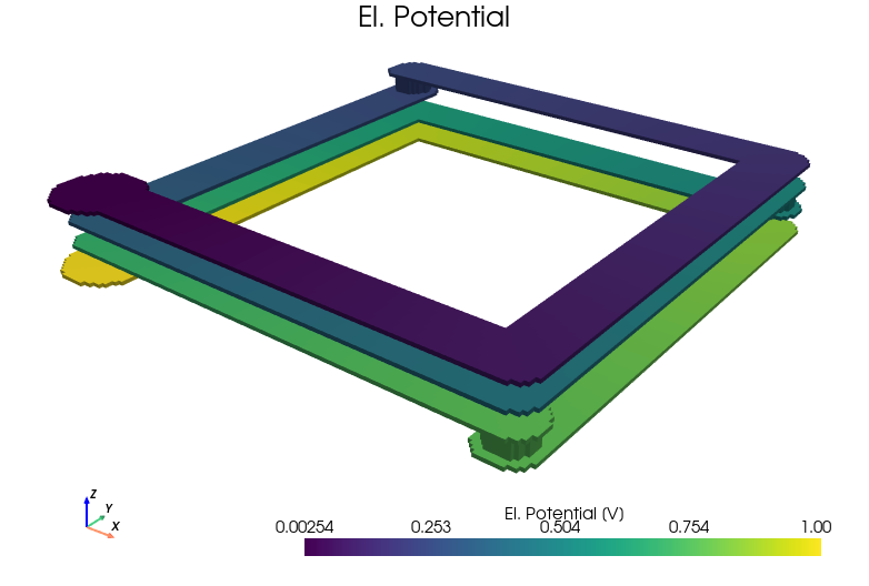
Plot showing the electric potential.
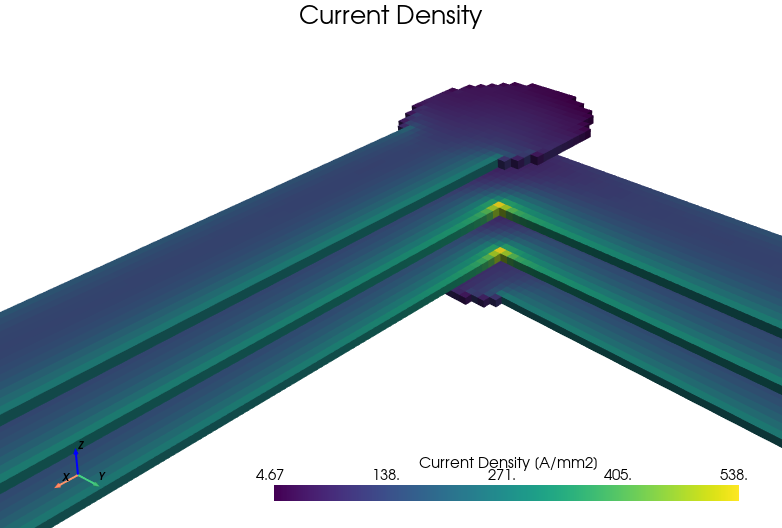
Plot showing the current density.
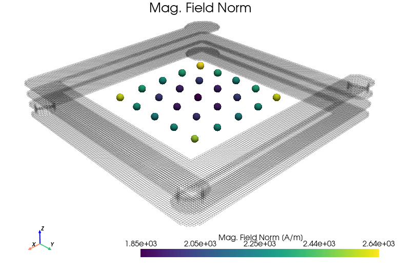
Plot showing the generated magnetic field.
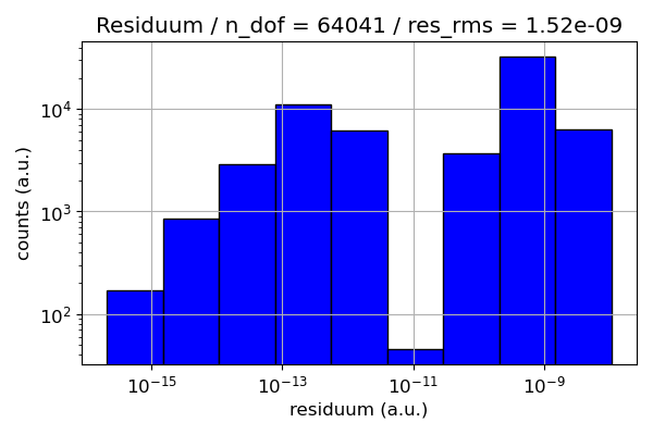
Plot showing the equation system residuum.